Goal

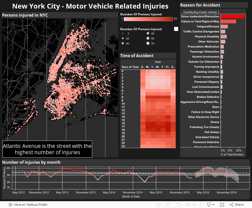
Since Bill de Blasio has taken office in 2013 one of his missions for his mayorship of New York City is to reduce the number of traffic-related injuries and fatalities in his "Vision Zero" campaign. An ambitious campaign to reach zero traffic injuries. I analyze data provided by NYC (you can dowload the dataset here), in order to determine whether the campaign was successful in reducing the number of traffic-releated injuries.

Tableau Visualization


The dashboard is posted on Tableau Public here.


Finding Trends


Dangerous Intersections

From the map on the dashboard, which shows the total number of injuries over the given data range on a map of NYC, we can see a number of locations of high injuries. This may suggest where the most dangerous intersections are in NYC and provide insight as to why there are accidents and whether or not Vision Zero is working, as well as point to where improvements could be made. Notable streets include 125th and 42nd st in manhattan, Eastern Parkway and Atlantic Ave in Brooklyn, and Woodhaven Blvd and Queens Blvd in Queens, to mention a few. All these roads are all arterial roads in NYC that have a large number of lanes and fast-moving traffic. Moreover, these intersections are also home to busy subway stops with express lines. At these points there is either a high concentration of pedestrian traffic, a high traffic flow rate of motor vehicles, or both.

From the map we can see that the most dangerous intersection in New York City is Flatbush aveune and Empire boulevard, an intersetion of two busy roads and also on the perimeter of New York City's second largest park, Prospect Park.


Dangerous Times

To explore further whether increases in pedestrian activity correlate to increases in traffic-related injuries, we can explore the common times in the day and year where injuries occur. The bottom graph of the dashboard shows the number of injuries over month. We can see a trend in the number of injuries versus month, and that in general, winter months, such as February and March, have less injuries in a given day, this may be because there are less pedestrians are on the street.

A trend line is included on the graph, however it has a high p-value and low R-squared value indicating it is not a good fit. This is liely due to the seasonality of the data, a more accurate trend would look at the same month over the various years, to remove the seasonality feature in the trend. Regardless, we see a slight negative slope, indicating a decrease in the number of injuries of around 131 per month. However, I stress that this is not statistically significant since the p-value is around 0.247. This is due to attempting to fit the data using linear regression when there is high variation and periodicity due to the month. The forecast in the graph does take seasonality into account, so the forecast looks plausible.

If we look at the number of injuries in a given time of day, shown in the middle graph of the dashboard, we can see that the most common time for an injury is between 8-9AM on weekdays and from 4-6PM on weekdays. This is when a large portion of the population are commuting to work, and again commuting home from work. Also we can note that Fridays from 2-7PM has a disproportionately large amount of injuries. This is likely due to people commuting home in what I describe as "weekend mode", and have a lowered state of focus on their commute home from work, excited for the weekend, resulting in a higher likelyhood of getting into an accident. Overall it seems there is a trend of the total number of injuries with number of pedestrians on the street, which are in the summer months and commuting hours.


Reasons for Accidents

Next, if we look at the reason for the collision we might be able to suggest opportunities of avoidance. We can see that the top 4 reasons for collisions are: "Driver inattention/distraction", "Failure to yield right-of-way", "Fatigued/drowsy", and "Traffic control disregarded". Altogether these account for almost 60% of the total injuries caused, and can be generally classified as accidents due to the driver's inattention.


Recommendations


Since Bill de Balsio's Vision Zero started in 2013 the number of traffic-related injuries has not decreased since 2013 by a statistically significant amount, so we cannot reject the null hypothesis. Moreover, I have identified some key features in the motor collision dataset that could help the Vision Zero campaign decrease the number of traffic-related injuries that occur in NYC. Based on these features I would make the following recommendations on where to focus efforts:

  • First, to target efforts on daily commuters during morning and evening rush hour, especially during the summer and fall months, since these time-frames account for a disproportionate number of the injuries that occur.

  • Second, targeting the arterial highways that run through the boroughs and neighbouring states.

  • Finally, by finding solutions to keep driver awareness and alertness.

One solution to these problems could be to engage drivers alertness using mobile LED signs, such as those often used to alert drivers of roadwork, repurposing them would be a quick and economical solution, and could be moved to intersections known for traffic-related injuries.

A longer term solution may be to change the traffic light signal pattern, such that either only cars can cross the intersection, or only pedestrians can cross. This would reduce the interaction bewteen motor vehicles and pedestrians which is a large source of injuries. This can be taken further, and a "scramble" crosswalk can be implemented, also known as a "Barnes dance". This solution was recently implemented in Los Angeles and is already seen as a great success. This solution is expensive however, but may be implemented at New York Cities most dangerous intersections first to effectively reduce traffic fatalities.


Analysis in R


Motivation

So we have seen using Tableau that we can display a large amount of information pertinent to the Vision Zero campaign in one interactive graphic. One thing I would further like to explore, however, is the time-dependence of the injuries over time. Namely, to explore the seasonality over time. While the Tableau software ouputs a convincing forecast, that does take into account the seasonality, using R to explore the detail will give a much deeper analysis that would be more suitable for a more techinal presentation, such as to other data scientists.

We load in the relevant packages in R

library(dplyr)
                  library(tidyr)
                  library(ggplot2)
                  library(lubridate)
                  library(caret)
                  library(DAAG)
                  library(forecast)
                  library(TTR)

The data is saved in a sqlite database, so in R we open a SQL connection. While I could use SQL qeries to access a subset of the data, since dplyr optimizes SQL queries under the hood.

VZCollision <- tbl(src_sqlite(path='VisionZeroDB.sqlite'),'VZCollision')
                  tidy.VZ <- VZCollision %>%
                    select(Date, PersonsInjured) %>%
                    filter(PersonsInjured > 0) %>%
                    group_by(Date) %>%
                    summarise(Total.Counts = sum(PersonsInjured))
                  tidy.VZ2 <- collect(tidy.VZ)
tidy.VZ2$Date <- as.Date(tidy.VZ2$Date, '%m/%d/%Y')
                  tidy.VZ2 <- arrange(data.frame(tidy.VZ2), Date)

We gather the data by the date, and count the number of nonzero injured persons. Now we have a tidy dataset, with one column containing the date, and the second column containing the total number of persons injured in that day.

It is a good question to ask why the data is even in a SQL database in the first place, since the total data is 162MB, and will easily fit in memory of even a modest laptop. The reason is because I find it a good habit to get into, loading, saving, and accessing SQL tables in databases. Moreover, loading in the full dataset, when I know I am only going to use a small subset, will take perhaps 30 seconds to 1 minute to load in, whereas loading in the data via an optimised SQL query will take less than 1 second.


Time-Series Analysis


In R we can easily plot the data and add a linear regression trend line with 95% confidence intervals using the ggplot library.

ggplot(data = tidy.VZ2, aes(x = Date, y = Total.Counts)) + geom_line() + geom_smooth(method = lm)

We apply simple linear model fit over the course of the entire data. To answer the question as to whether the Vision Zero campain is working this is a good way to quickly find out in the macro sense. Because of the high seasonality in the data it makes the most sense to explore yearly trends in the data to rule out any underlying factors.

In R we use the lm function to perform linear regression on the dataset.

lmfit <- lm(tidy.VZ2$Total.Counts ~ tidy.VZ2$Date)
lmfit
Call:
lm(formula = tidy.VZ2$Total.Counts ~ tidy.VZ2$Date)

Coefficients:
  (Intercept)  tidy.VZ2$Date
    1.192e+02     -8.119e-04  


We can see from from the linear regression that the number of persons injured does decrease over time, but it is at the rate of 0.0008119 persons per day, or decreases by roughly one person every 3 years. So I would argue, that Vision Zero has not been successful in decreasing the number of traffic injuries.

We can perform a t-test on the data to determine whether the number of injuries is correlated with the date. Instinctively we would think it is because, while the linear regression line is almost flat, there appears to be some time-dependent seasonality to the data, so the p-value should be very small.

t.test(row_number(tidy.VZ2$Date), tidy.VZ2$Total.Counts)
    Welch Two Sample t-test

data:  row_number(tidy.VZ2$Date) and tidy.VZ2$Total.Counts
t = 56.679, df = 1472.4, p-value < 2.2e-16
alternative hypothesis: true difference in means is not equal to 0
95 percent confidence interval:
 605.7602 649.1920
sample estimates:
mean of x mean of y
 733.5000  106.0239 


Indeed the p-value is less than 0.05 so the correlation is statistically significant. Ideally we want to look at the over the same day or week of the year, and see how that varies over the course of the years. However, there is only 3 complete years. so any trends observed may not be relevant.

We can aggregate by month and plot, to see the seasonality of the data over the years. By plotting the data we may be able to see any decreases in the number of injuries for each month.

tidy.VZ3 <- tidy.VZ2 %>% mutate(Year = year(tidy.VZ2$Date), Month = month(tidy.VZ2$Date),
                               Week = week(tidy.VZ2$Date), Day = day(tidy.VZ2$Date),
                               Wday = wday(tidy.VZ2$Date)) %>% ungroup()
Injuries.By.Month.Year <- tidy.VZ3 %>%
  group_by(Month, Year) %>%
  summarise(Total.Counts = sum(Total.Counts))

ggplot(data = Injuries.By.Month.Year, aes(x= Month, y = Total.Counts, color = as.factor(Year)))
  + geom_line()

To address the obvious first, the large dip for July 2016 occurs because the motor vehicle collision dataset only goes up to July 5th 2016, so there is only a small amount of data for this particular month.

To better fit the data we can take the weekday (1-7), day of the month (1-31), week (1-52), and month (1-12) into account, and use multivariate nonlinear regression. Moreover, because many of these variables are periodic in nature, i.e. the end of the week is the beginning of the next week, we can map these onto periodic funtions. In this case we use sin and cosine functions.

To build accurate predictions and prevent overfitting we perform a split on the dataset, we train on the the first 90%, and leave 10% for testing.

dataPartition <- as.integer(.9*length(tidy.VZ3$Total.Counts))
df_train <- tidy.VZ3[ 1:dataPartition,]
df_test  <- tidy.VZ3[-(1:dataPartition),]
fit.mvlm <- lm(data = df_train, Total.Counts~ Year * Date * (sin(2*pi*Day/31) + cos(2*pi*Day/31)) *
                 (sin(2*pi*Month/12) + cos(2*pi*Month/12)) * (sin(2*pi*Week/52) + cos(2*pi*Week/52)) *
                 (sin(2*pi*Wday/7) + cos(2*pi*Wday/7)))


We can then plot the fitted data in red, along with the original data in black, and the forecasted data in green.

ggplot() + geom_point(data = tidy.VZ3, aes(x = Date, y = Total.Counts)) +
  geom_line(data = fit.mvlm, aes(x = tidy.VZ3$Date[1:dataPartition], y = fit.mvlm$fitted.values), color = 'red') +
  geom_line(aes(x = tidy.VZ3$Date[-(1:dataPartition)], y = predict.lm(fit.mvlm, df_test)), color = 'green')

RMSE(predict.lm(fit.mvlm, df_test), tidy.VZ3$Total.Counts[-(1:dataPartition)])
[1] 34.37359


The root mean squared error (RMSE) is quite high on the test set, since the average number of injuries per day is 119. This is likely due to overfitting of the data, due to the high number of variables.


Time-Series Decomposition


A better method to fit the time series data is to use the Holts-Winter (HW) method. There are 3 components that the HW method can determine that makes this a suitable method to analyse this dataset. The components the HW method will determin are:

  • The current underlying number of injries. This is the level that remains after we have deseasonalized the number of injuries and attempted to remove the effect of random factors (noise)

  • The current trend in the number of injuries. This is the change in the underlying level that we expect to occur between now and the next day. For example, if we estimate our current level is 119 injured persons and we expect this to be 123 the next day, then our estimated trend is +4 units.

  • The seasonal index for the day we are forecasting. Let’s say our estimate is 1.02; this means that we expect the number of injuries in the day to be 2% above that day's underlying level, showing that there will be relatively more injuries on the day.

We can decompose the data in R and plot each component.

tsTC <- ts(tidy.VZ3$Total.Counts, frequency = 365, start=c(2012, 7))
                  TCComp <- decompose(tsTC)
                  plot(TCComp)

From the decomposition we can see that the trends, which would show the long term effects are very small, and only vary by about 8 from the minimum the maximum, this agrees with the simple linear model that shows no significant long term changes in the number of persons injured.

The seasonal changes are much larger in magnitude, and the random components are even larger. This tells us that it will be hard to accurately predict the number of injuries over time, and in best case we might expect low p-values, where the seaonal and underlying trends are well predicted, but a R^2 value that may not be that high, due to the large random fluctuations.

TCForecasts <- HoltWinters(tsTC)
TCForecasts
Holt-Winters exponential smoothing with trend and additive seasonal component.

Call:
HoltWinters(x = tsTC)

Smoothing parameters:
 alpha: 0.03054984
 beta : 0
 gamma: 0.5717582

Coefficients:
              [,1]
a    103.196962284
b     -0.003571926
s1    14.943176086
...  ...
s365 -17.717592045

The estimated values from the HW exponential smoothing of alpha, beta and gamma are 0.031, 0.00, and 0.57, respectively. The value of alpha (0.031) is very low, indicating that the estimate of the level at the current time point is based almost entirely upon recent observations and little observations in the more distant past. The value of beta is 0.00, indicating that the estimate of the slope b of the trend component is not updated over the time series, and instead is set equal to its initial value. This makes good intuitive sense, as the level changes quite a bit over the time series due to seasonal changes, but the slope b of the trend component remains roughly the same. In contrast, the value of gamma (0.57) indicates that the estimate of the seasonal component at the current time point is based equally upon both recent observations, and observations from the past.

We can use this model to forcast the data for future predictions. We predict the number of injuries for the next year.

TCFutForecasts <- forecast.HoltWinters(TCForecasts, h = 365)
plot.forecast(TCFutForecasts)

In the forecast, the blue area is the 85% confidence interval, gray is 90%, and light gray is 90%. We can see that forecast seems convincing in that it continues the underlying trend, similar to the linear regression model, and also conserves the seasonal data.


Conclusion

From the time series analysis we have confirmed the analysis performed in Tableau, and the thesis of this project: Vision Zero has been ineffective in reducing the number of injuries in New York City. Moreover in this recent analysis we have examined the seasonal trends in the data using a Holts-Winter Method, whereas mulitivariate linear regression did not perform that well. We have shown the the number of persons injured is dominated by seasonal and random data, and the underlying trend is fairly constant, which agrees with our linear regression model. The Holts-Winter method is useful because it splits the data into interpretable components and those underlying and seasonal trends can be analysed separately.

Ultimately the methods used here may be applied in many disciplines which display seasonal time-series data, such as business sales trends, weather predictions, or stock market analysis, and is useful for providing an interpretable decomposition of the data at hand.