Goal

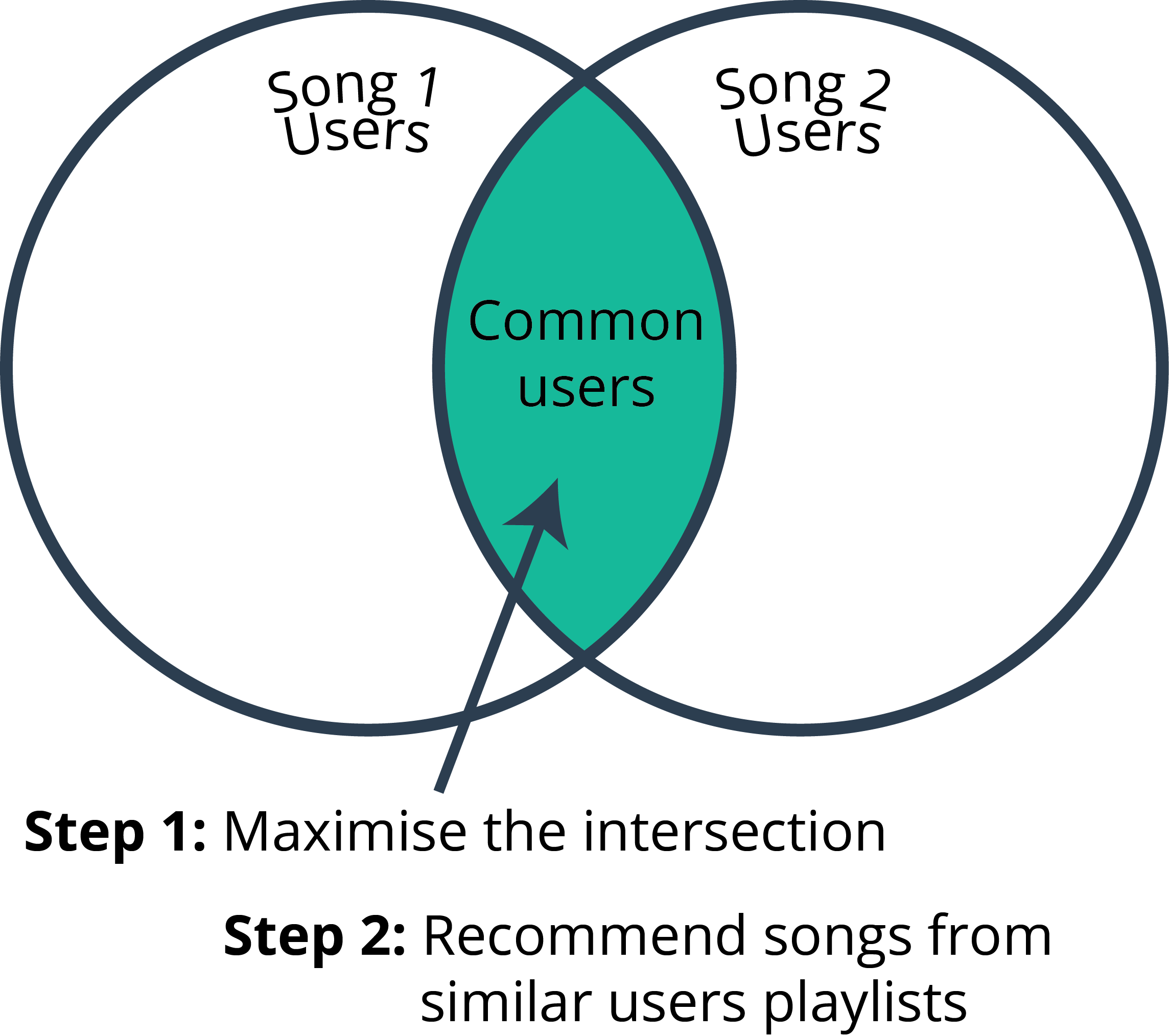
The goal is to build a music recommendation system that can provide custom playlists for individual users based on collaborative and metadata filtering. Currently music service providers have generic (and popular), mood-based playlists, that are the same for all users. Here, I suggest improvements to these playlists by offering custom options for each user based on song metadata.

The complete code can be found on github here.

Approach

I will first determine the the best method to recommend songs to users based on the most listened songs, song-song similarity, and user-user similarity. This will form the basis of the playlist creator. The specific playlist will then be constructed from these songs, since the ultimate goal is to create a playlist of songs the user likes. The songs will be chosen based on the type of playlist, i.e., workout, chillout, discover new artists, etc, and the songs are chosen based on their metadata.

The data comes from the Million Song Dataset which has metadata on 1 million songs. The metadata comes from the The Echo Nest, that is know taken over by Spotify earlier in 2016. The dataset of users listener histories comes from kaggle that had a competition on the subject a few years ago. The listening history was kept hidden by kaggle, so half the total data was not available to me, however this can be supplemented by the million song dataset that can be found on the UCI Machine Learning Repository. However for a single machine the kaggle dataset with 110000 unique users and 149029 unique songs is enough to test hypotheses.


Exploratory Data Analysis


Exploratory data analysis is performed in R to get a general feel for the data.

See here ▼

# Load in libraries
library(readr)
library(dplyr)
library(tidyr)
library(RSQLite)
library(ggplot2)

# Load in data and create data frames
# User data
user_data <- as.data.frame(read.table('data/kaggle/kaggle_users.txt'))
colnames(user_data) <- c('User_ID')
user_data <- mutate(user_data, UID = row(user_data))

# Songs data
song_data <- as.data.frame(read.table('data/kaggle/kaggle_songs.txt'))
colnames(song_data) <- c('Song_ID', 'index')

# triplets in the form (User_ID, Song_ID, number of plays)
triplets <- as.data.frame(read_table('data/kaggle/kaggle_visible_evaluation_triplets.txt'))
colnames(triplets) <- c('User_ID', 'Song_ID', 'Plays')

# dataframe to convert song ID to track ID since metadata is from different source
song2track <- as.data.frame(read.table('data/kaggle/taste_profile_song_to_tracks.txt', fill= TRUE))
colnames(song2track) <- c('Song_ID', 'Track_ID')

# Join dataframe
totdf <- left_join(triplets, song2track, by = "Song_ID")

# Load data from databases using SQLite
con = dbConnect(drv=RSQLite::SQLite(), dbname="data/MillionSongSubset/AdditionalFiles/track_metadata.db")
songs <- dbGetQuery(con, 'SELECT * FROM songs')

con_meta = dbConnect(drv=RSQLite::SQLite(), dbname="song_metadata.sqlite")
song_metadata <- dbGetQuery(con_meta, 'SELECT track_id, loudness, time_signature, song_hotttnesss FROM song_metadata')

con_simArt = dbConnect(drv=RSQLite::SQLite(), dbname="data/MillionSongSubset/AdditionalFiles/artist_similarity.db")
sim_Artists <- dbGetQuery(con_simArt, 'SELECT * FROM songs')

# Join all data sources and remove unnecessary columns
totdf2 <- totdf %>% left_join(songs, by = c('Track_ID' = 'track_id')) %>%
  filter(!is.na(title)) %>%
  left_join(song_metadata, by = c('Track_ID' = 'track_id')) %>%
  select(-song_id, -track_7digitalid, -shs_perf, -shs_work)

# Exploratory data analysis
popular_songs <- totdf2 %>%
  dplyr::group_by(title, artist_name) %>%
  dplyr::summarise(Total.plays = sum(Plays)) %>%
  dplyr::arrange(desc(Total.plays)) %>%
  dplyr::top_n(100)

popular_artists <- totdf2 %>%
  dplyr::group_by(artist_name) %>%
  dplyr::summarise(Total.plays = sum(Plays)) %>%
  dplyr::arrange(desc(Total.plays)) %>%
  dplyr::top_n(100)

hottest_artists<- totdf2 %>%
  dplyr::select(artist_name, artist_hotttnesss) %>%
  dplyr::distinct() %>%
  dplyr::arrange(desc(artist_hotttnesss)) %>%
  dplyr::top_n(100)

hottest_songs <- totdf2 %>%
  dplyr::select(artist_name, title, song_hotttnesss) %>%
  dplyr::distinct() %>%
  dplyr::arrange(desc(song_hotttnesss)) %>%
  dplyr::top_n(100)

songs_per_user <- totdf2 %>%
  dplyr::select(User_ID, Song_ID) %>%
  dplyr::group_by(User_ID) %>%
  dplyr::summarize(Total.Songs = n()) %>%
  dplyr::arrange(Total.Songs) %>%
  dplyr::group_by(Total.Songs) %>%
  dplyr::summarise(Total.Count = n()) %>%
  dplyr::mutate(Cum.Sum = cumsum(Total.Count))

ggplot() + geom_line(data = songs_per_user, aes(x = Total.Songs, y = Cum.Sum/max(Cum.Sum)))

users_per_song <- totdf2 %>%
  dplyr::select(User_ID, Song_ID) %>%
  dplyr::group_by(Song_ID) %>%
  dplyr::summarise(Total.Users = n()) %>%
  dplyr::group_by(Total.Users) %>%
  dplyr::summarise(Total.Count = n()) %>%
  dplyr::mutate(Cum.Sum = cumsum(Total.Count))

ggplot() +
  geom_line(data = users_per_song, aes(x = Total.Users, y = Cum.Sum/max(Cum.Sum))) +
  scale_x_log10()

ggplot() + geom_histogram(data = filter(totdf2, year>1900), aes(x = year), binwidth = 1,
                          fill = '#18BC9C', color = '#2C3E50') +  xlim(1940,2012) +
  labs(title = 'Number of Songs per Year', x = 'Year', y = 'Count')+
  theme(plot.title = element_text(size=22), axis.text.x = element_text(size=18),
        axis.text.y = element_text(size=18), text = element_text(size = 20))

ggplot(data = filter(totdf2, year>1900),
       aes(x = as.factor(year), y = loudness) ) + geom_boxplot(aes(fill = (year))) +
  scale_fill_gradient(low = 'yellow', high = 'red') +
  scale_x_discrete(breaks = seq(1920, 2010, 10)) +
  labs(title = 'Loudness vs Year', x = 'Year', y = 'Loudness (dB)')+
  theme(plot.title = element_text(size=22), axis.text.x = element_text(size=18),
        axis.text.y = element_text(size=18), text = element_text(size = 20))


Most Popular Songs

Popular songs based on total numer of plays across all users.


Artist Name Song Title Total Plays
Dwight Yoakam You're The One 35432
Björk Undo 33179
Kings Of Leon Revelry 24359
Barry Tuckwell/Academy of St Martin-in-the-Fields/Sir Neville Marriner Horn Concerto No. 4 in E flat K495: II. Romance (Andante cantabile) 17115
Florence + The Machine Dog Days Are Over (Radio Edit) 14279
OneRepublic Secrets 12392
Sam Cooke Ain't Misbehavin 11610
Tub Ring Invalid 10794
Lonnie Gordon Catch You Baby (Steve Pitron & Max Sanna Radio Edit) 10515
Five Iron Frenzy Canada 9921


Hotttest Songs

Song hotttnesss[sic] is a metric defined by how much buzz the song is getting right now. This is derived from many sources, including mentions on the web, mentions in music blogs, music reviews, play counts, etc.


Artist Name Song Title Hotttnesss Value
Florence + The Machine Dog Days Are Over (Radio Edit) 1
OneRepublic Secrets 1
Pearl Jam Black 1
Modest Mouse Float On 1
Kings Of Leon Use Somebody 1
Jimmy Eat World The Middle 1
B.o.B Nothin' On You [feat. Bruno Mars] (Album Version) 1
MIKA Grace Kelly 1
Vampire Weekend Cape Cod Kwassa Kwassa (Album) 1
Train Marry Me 1


Interestingly, despite song hotttness being defned from the amount of buzz the song is currently getting, we see songs that are relatively old, such as Pearl Jam's 'Black', and Jimmy Eat World's 'The Middle', that are from 1991 and 2001 respectively.


Total songs in the dataset versus the year they were released.


Cumulative distribution function showing total number of songs have listened by less than x users. For example, cumulative sum for 10 total users is around 137,000, this means that 137,000 songs have been listened to by at most 10 unique users.


Cumulative distribution function of the total number of users have listened to less than x total songs. For example, the cumulative sum for 20 total songs is around 90,000, which means that 90,000 users have listened to at most 20 unique songs.


Loudness versus year. Although we acknowledge that comparing features over time may not help in recommending songs, it may be valuable for visualizing trends in data and discovering any possible insights. One relationship we see confirms the "loudness wars", that refers to the trend of increasing the audio levels of music. The concept derives from the principle that if the audio levels are higher than other songs, when played on the radio the song will be louder, and listeners may pay attention to the song more. This is captured below in the boxplot graph.


Methods to Recommend Songs


Cosine Similarity

When dealing with a large number of users and a large number of songs and find similarities between users or songs things can quickly get out of hand. For example, to calculate the song similarity between all songs we could go through each song and calculate its similarity with each other song, however that would involve nested for loops with \(\frac{n(n-1)}{2} \) operations. Since there are 149029 unique songs in the data set, this equates to 11104746906 operations. While this is highly parallelizable, for optimal use of resources, we use linear algebra.

To solve the similarity between users and songs we construct a sparse matrix, \(R(i,j)\), that is \(m\times n\), where m is the total number of users, and n is the total number of songs. The entry of the matrix for user i at song j represents the relative number of plays that of the song compared to the total number of songs the user listens to, i.e., is the user listens to a song 6 times out of listening to 60 songs total, the relative play would be 0.1. We use relative plays as it will make constructing the similarity matrices easier.

We define the cosine similarity for two arbitrary vectors as:

Cosine similarity = \(\frac{u^Tv}{\lVert u \rVert \lVert v \rVert}\)

The user-user similarity matrix can be computed as:

User-user similarity = \( RR^T\)

which produces a symmetric \(m\times m\) matrix, where \(m\) is the total number of users. The item-item similarity can be calculated in a similar way:

Item-item similarity = \( R^TR\)

which produces a symmetric \(n\times n\) matrix, where \(n\) is the total number of songs.


Evaluation Metric

We use the mean average precision (MAP) as the evaluation metric.

For any k, define the precision-at-k \(P_k\) as the proportion of correct recommendations within the top-k of the predicted ranking:

\( P_k(u,y)=\frac{1}{k}\sum_{j=1}^kM_{u,y(j)}\),

next we take the average of the computed precisions:

\( AP(u,y)=\frac{1}{n_u}\sum_{k=1}^\tau P_k(u,y)\times M_{u,y_u(k)}\)

where \(\tau\) is the threshold that represents how many of the top predictions in \(y_u\) to include and \(n_u\) is the number of songs in the users hidden history.

Finally, we take the average over all users precisions:

\( MAP = \frac{1}{m}\sum_{u}AP(u,y_u)\)

The R functions for the evaluation metrics are shown below:

average_precision_at_k <- function(k, actual, predicted){
  score <- 0.0
  cnt <- 0.0
  for (i in 1:min(k,length(predicted)))
  {
    if (predicted[i] %in% actual && !(predicted[i] %in% predicted[0:(i-1)]))
    {
      cnt <- cnt + 1
      score <- score + cnt/i
    }
  }
  score <- score / min(length(actual), k)
  return(score)
}

mAP = mean(average_precision_at_k(500, valid_data, predicted_songs))


Strategy - Recommend top 500

A simple strategy would be to suggest the same top 500 most played songs to all users.

To do this, first, we load in the relevant libraries, and construct the training and validtion datasets. For details on the initial loading of the data from the text files and SQLite databases the R code above.

library(readr)
library(dplyr)
library(tidyr)
library(Matrix)
library(plyr)
library(pbapply)

# Load in data
triplets <- as.data.frame(read_table('data/kaggle/kaggle_visible_evaluation_triplets.txt'))
colnames(triplets) <- c('User_ID', 'Song_ID', 'Plays')

# Split data into train and validation set
set.seed(666) # reproducibility
train_data <- triplets %>%
  dplyr::group_by(User_ID) %>%
  dplyr::sample_frac(0.8) %>%
  dplyr::ungroup()

valid_data <- setdiff(triplets, train_data)


The top 1000 songs are chosen based on total number number of plays across all users.

# baseline is to recommend top n most played songs,
top1000songs <- train_data %>%
  dplyr::group_by(Song_ID) %>%
  dplyr::summarise(Total.Plays = sum(Plays)) %>%
  dplyr::arrange(desc(Total.Plays)) %>%
  dplyr::top_n(1000) %>%
  dplyr::ungroup()

getBaseline_AveragePrecision(user){
  actual.songs <- filter(valid_data, User_ID == unique_users$User_ID[user])
  avg.Pres <- average_precision_at_k(k=500, actual = actual.songs$Song_ID,
                                     predicted = top1000songs$Song_ID[1:500])
  return(avg.Pres)
}

mAP_baseline <- pbsapply(seq(nrow(multMat2)), getUser_Average_Precision)


Strategy - Recommend songs by finding similar songs to songs in users list of listened songs

Two songs are similar if they have many users in common that listen to both.

This is achieved in R by creating a sparse matrix, and performing the operations on the sparse matrix.

# Create data frames of the unique songs and users
unique_users <- unique(train_data$User_ID)
unique_songs <- unique(train_data$Song_ID)

unique_users <- as.character(unique_users)
unique_songs <- as.character(unique_songs)

# Create new column where user/song ID -> unique numeric
unique_users <- cbind(unique_users, as.numeric(seq(nrow(as.data.frame(unique_users)))))
unique_songs <- cbind(unique_songs, as.numeric(seq(nrow(as.data.frame(unique_songs)))))

colnames(unique_users) <- c('User_ID', 'UID')
colnames(unique_songs) <- c('Song_ID', 'SID')

train_data$User_ID <- as.character(train_data$User_ID)
train_data$Song_ID <- as.character(train_data$Song_ID)

# Join datasets
train_data_2 <- train_data %>%
  dplyr::left_join(as.data.frame(unique_users), by = 'User_ID') %>%
  dplyr::left_join(as.data.frame(unique_songs), by =  'Song_ID') %>%
  dplyr::group_by(User_ID) %>%
  dplyr::mutate(Relative.Plays = Plays/sum(Plays))

# remove all NAs
train_data_2[is.na(train_data_2)] <- 0

# Create sparse matrix
sparse_rating_df <- sparseMatrix(i = as.numeric(train_data_2$UID),
                                 j = as.numeric(train_data_2$SID),
                                 x = train_data_2$Relative.Plays)


The method used to recommend the songs will be to recommend songs that are similar to songs already in the users list of listened songs. This is shown using the Venn diagram below.


The R code to achieve the item-item similarity is as follows:

# Song similarity matrix
multMat1 <- t(sparse_rating_df) %*% (sparse_rating_df)

# Get top 500 similar songs of a given song
gettop500simSong <- function(song){
  user_sim <- multMat1[song,]
  user_sim <- as.data.frame(cbind(user_sim, seq(length(user_sim))))
  colnames(user_sim) <- c('Similarity', 'SID')
  user_sim <- user_sim %>%
    dplyr::left_join(unique_songs, by = 'SID') %>%
    dplyr::arrange(desc(Similarity)) %>%
    dplyr::top_n(500, Similarity)
  return(user_sim)
}

# Get average precision of user via song similarity
getSong_Average_Precision<- function(user){
  # Get the visible song in users song list
  songs <- train_data_2 %>%
    filter(UID == user) %>%
    select(SID)

  # If SID is of factor class change to integer
  if (class(songs$SID) == "factor"){
    songs$SID <- as.integer(levels(songs$SID))[songs$SID]
  }

  # Go through songs and get 500 most similar songs
  top500total <- ldply(songs$SID, gettop500simSong) %>%
    anti_join(songs, by = 'SID') %>% # remove songs already in users song list
    distinct() %>%                   # remove duplicates
    arrange(desc(Similarity)) %>%    # order by similarity
    top_n(500, Similarity)           # take top 500

  # Get actual songs from validation datset
  actual.songs <- filter(valid_data, User_ID == unique_users$User_ID[user])

  # Calculate average precision
  avg.Pres <- average_precision_at_k(k=500, actual = actual.songs$Song_ID, predicted = top500total$Song_ID)
  return(avg.Pres)
}

mAP <- mean(pbsapply(seq(nrow(multMat1)), getSong_Average_Precision))


Strategy - Recommend songs by finding similar users and selecting songs in their list of listened songs

Two users are similar if they have listened to many of the same songs. The user-user similarity is calculated in a similar way to the item-item similarity. After each users recommendations the songs are ordered in termes of total plays. The Venn diagram of the strategy is shown below.


The R code to achieve this is as follows:

# User similarity matrix
multMat2 <- sparse_rating_df %*% t(sparse_rating_df)

# Function that recommends songs based on 2 users song list
recommend_by_user <- function(user1, user2){
  # Get song intersection of 2 users
  user1.songs <- train_data %>%
    dplyr::filter(User_ID == user1) %>%
    dplyr::select(Song_ID, Plays)
  user2.songs <- train_data %>%
    dplyr::filter(User_ID == user2) %>%
    dplyr::select(Song_ID, Plays)

  # Get songs in user2, that not in user1
  recommend.songs <- dplyr::anti_join(user2.songs, user1.songs,
                                      by = 'Song_ID') %>%
    dplyr::arrange(desc(Plays)) %>%  # sort by number of plays
    dplyr::select(-Plays)
  return(recommend.songs)
}

getUser_Average_Precision<- function(user){
  # Get top 100 unique users
  user1_sim <- multMat2[user,]
  user1_sim <- as.data.frame(cbind(user1_sim, seq(length(user1_sim))))
  colnames(user1_sim) <- c('Similarity', 'UID')
  user1_sim <- user1_sim %>%
    dplyr::arrange(desc(Similarity)) %>%
    dplyr::top_n(100, Similarity) %>%
    dplyr::left_join(unique_users, by = 'UID')

  # Initialsize empty data frame
  rec.songs <- data.frame()
  i = 1
  while(nrow(rec.songs) < 500){
    # Recommend songs if they have any songs in common (similarity > 0)
    if(user1_sim$Similarity[i] > 0.00000){
      new.songs <- recommend_by_user(user1_sim$User_ID[user], user1_sim$User_ID[i])
      rec.songs <- unique(rbind(rec.songs, new.songs))
    }
    # otherwise choose from top 1000 songs
    else{
      new.songs <- as.data.frame(top1000songs$Song_ID[1:(1000-nrow(rec.songs))+1],
                                 stringsAsFactors = FALSE)
      colnames(new.songs) <- 'Song_ID'
      rec.songs <- unique(rbind(rec.songs, new.songs))
    }
    i = i + 1
  }

  # Get actual songs from validation datset
  actual.songs <- filter(valid_data, User_ID == unique_users$User_ID[user])

  # Calculate averag precision
  avg.Pres <- average_precision_at_k(k=500, actual = actual.songs$Song_ID, predicted = rec.songs$Song_ID)
  return(avg.Pres)
}

mAP <- mean(pbsapply(seq(nrow(multMat2)), getUser_Average_Precision))


Results


In the results shown, k-fold cross validation is used, for k=5. The MAP for each of the strategies is shown below.


We can see that item/item similarity has the largest MAP score, slightly outperforming the user-user similarity strategy. In terms of run time, the base-line strategy is unsurprisingly the quickest, at around 0.72 seconds/user, followed by item-item similarity at around 4.23 seconds per user, and finally the user-user similarity was significantly slower at 121.2 seconds/user. This may be due to the user-user similarity matrix, while smaller than the item-item similarity (1100002 vs 1490292), it is not as sparse, so sorting through the matrix, in looking for common users, as well as allocating memory is more expensive.


Recommending Songs based on Metadata


Discovering new artists

Since item/item similarity was gave the best results and was much quicker to process this is the stratey we will continue with, though the same recommendation methods can be used with the user/user similarity.

Since there are no correct answers, evaluation metrics are redundant, and A/B/n testing would be more appropriate.

To discover new artists we follow a similar method however in the top 500 similar artists we will order in the list in terms of artist ascending familiarity, and suggest those at the top first. The 'artist familiarity' corresponds to how well known in artist is. You can look at familiarity as the likelihood that any person selected at random will have heard of the artist. Kanye West has a familiarity close to 1, while a band like ‘Hot Rod Shopping Cart’ has a familiarity close to zero. In this way songs are both similar to songs in the users lists of listened songs, and unlikely to be heard by the user.

This can be achieved using the R code below.

discoverNewSongs<- function(user){
  # Get users songs
  usersongs <- train_data_2 %>%
    filter(UID == user) %>%
    select(SID)

  # If SID is of factor class change to integer
  if (class(usersongs$SID) == "factor"){
    usersongs$SID <- as.integer(levels(usersongs$SID))[usersongs$SID]
  }

  # Get top 500 similar songs for each song in user song list
  top500total <- ldply(usersongs$SID, gettop500simSong) %>%
    dplyr::anti_join(usersongs, by = 'SID') %>%                 # remove songs already in song list
    dplyr::distinct() %>%                                       # remove duplicates
    dplyr::top_n(500, Similarity) %>%                           # take top 500 based on similarity
    dplyr::left_join(songs, by = c('Song_ID' = 'song_id')) %>%  # join with metadata dataset
    dplyr::arrange(artist_familiarity) %>%                      # sort based on artist familiarity
    dplyr::select(artist_name, title, artist_familiarity, Song_ID)
  return(top500total)
}


Playlists to chillout/workout to

Many songs from chillout playlists, such as those found on Spotify or last.fm have slow and easy-going, characterized by a low tempo that will relax the listener. Alternatively, if listeners want to get motivated to workout they may want listen to songs with high tempo that will get their heartrate up. This can be done with the following code:

# Find songs with low tempo
downbeatSongs<- function(user){
  # Get users songs
  usersongs <- train_data_2 %>%
    filter(UID == user) %>%
    select(SID)

  # If SID is of factor class change to integer
  if (class(usersongs$SID) == "factor"){
    usersongs$SID <- as.integer(levels(usersongs$SID))[usersongs$SID]
  }

  # Get top 500 similar songs for each song in user song list
  top500total <- ldply(usersongs$SID, gettop500simSong) %>%
    dplyr::distinct() %>%                                 # Remove duplicates
    dplyr::top_n(500, Similarity) %>%                     # get 500 most popular songs
    dplyr::left_join(song2track, by = 'Song_ID') %>%      # to convert song_id to trackid
    dplyr::left_join(song_metadata, by = c('Track_ID' = 'track_id')) %>% # join with metadata
    dplyr::arrange(tempo) %>%                             # order with respect to tempo
    dplyr::select(Song_ID, tempo) %>%                     # select releveant columns
    dplyr::filter(!is.na(Song_ID))                        # remove NAs
  return(top500total)
}

# Find songs with high tempo
upbeatSongs<- function(user){
  usersongs <- train_data_2 %>%
    filter(UID == user) %>%
    select(SID)

  # If SID is of factor class change to integer
  if (class(usersongs$SID) == "factor"){
    usersongs$SID <- as.integer(levels(usersongs$SID))[usersongs$SID]
  }

  # Get top 500 similar songs for each song in user song list
  top500total <- ldply(usersongs$SID, gettop500simSong) %>%
    dplyr::distinct() %>%                                 # Remove duplicates
    dplyr::top_n(500, Similarity) %>%                     # get 500 most popular songs
    dplyr::left_join(song2track, by = 'Song_ID') %>%      # to convert song_id to trackid,
    dplyr::left_join(song_metadata, by = c('Track_ID' = 'track_id')) %>% # join with metadata
    dplyr::arrange(desc(tempo)) %>%                       # order with respect to tempo
    dplyr::select(Song_ID, tempo) %>%                     # select releveant columns
    dplyr::filter(!is.na(Song_ID))                        # remove NAs
  return(top500total)
}


In this application it doesn't matter if the songs are already in the users list of listened songs, unlike for recommending new music.

This serves as a good template for A/B/n testing, creating indices based on a variety of metadata may also be used, for example a workout index may be defined as the \(WI = \log(tempo\times danceability)\), where the danceabilty is defined from the Spotify/echonest API. A/B testing can by varying the indices created, selecting songs based on the indices. The best index can be determined based on user feedback, such as number of plays, shares, or follows of the playlist.


Conclusion

Overall, a successful recommendation system is made and has been applied to create custom mood-based playlists ready for A/B/n testing. It is shown that recommendation system based on item-item gives the largest mean average precision for the dataset. All strategies can be combined with different weights, however this in unrealistic with a single machine. Other methods to recommend songs is to find the user-user and item-item similarity via singular value decomposition, as this is fast and efficient, yet has a tendency to overfit, without regularization.