Recommender Systems

Content vs Collaborative

Content

Recommending items based on similarities between their features

For in the case of this recommending beer the features may be the proprtion of ingredients, colour, clarity, alcohol content, bitterness, etc. One beer is similar to another if it has many of the same features in common.

Pro: It can be useful in the interest of the "cold-start" problem, in which you may not have any user feedback.

Con: Doesn't take user information into account.

Collaborative

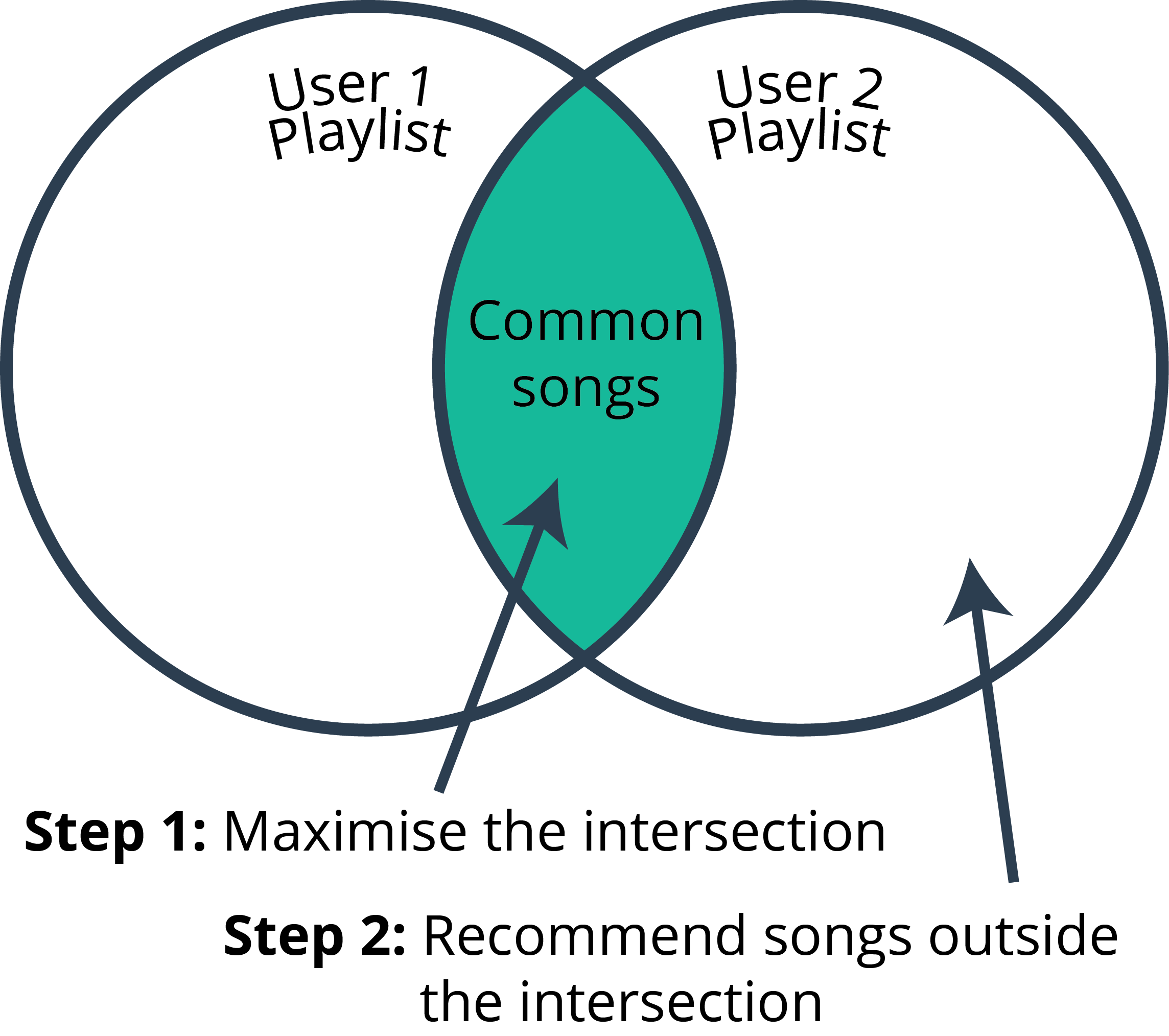
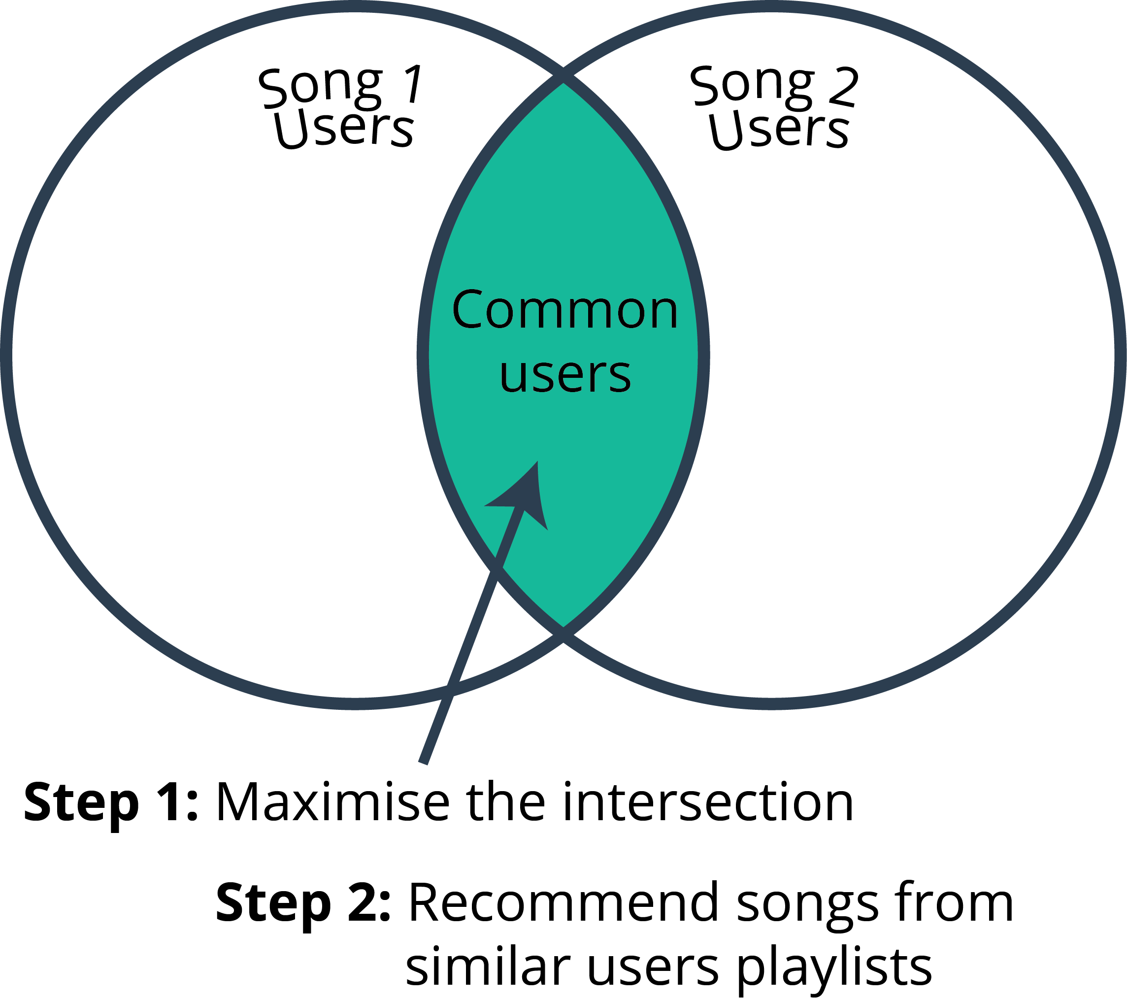
Collaborative filtering approaches building a model from a user's past behavior (items previously purchased or selected and/or numerical ratings given to those items) as well as similar decisions made by other users. This model is then used to predict items (or ratings for items) that the user may have an interest in.

Pro: No need to know about item content.

Pro: "Item cold-start" problem is avoided.

Pro: User interest taken into consideration.

Pro: Can capture subtle relationships.

Con: Usually deal with large, sparse matrices.

Con: Grey sheep whose taste and preference do not consistently agree with other users' preference are to to recommend for.

Con: Grey sheep whose taste and preference do not consistently agree with other users' preference are to to recommend for.

Explicit vs Implicit

Explicit

Explicit user preference requires user input, such as the ratings of movies on netflix.

Implicit

Another, more subtle way to passively guage a users preference for an item, is to look implicit factor such as purchase history, watching habits and browsing activity. For example, if a person has purchased a large amount of beer, or listened to a song a large number of times, we can implicitly infer that the user likes this particular beer or song, without explicitly asking them for their rating on the item.

Sparse Matrices

Sparse matrices are your friend. In python they help you efficiently work with large matrices that are mostly nonzeros. For example, in the case of recommending beers, it is highly unlikely that most of the users have tried, letalone rated, most of the beers in the dataset. As such the generated 2D matrix of unique users and unique beers will be mostly sparse.

In python they are in the scipy.sparse library. They come in a number of flavours that can be explored on scipy's webpage here.

beer_data = pd.read_csv('beer_reviews/beer_reviews.csv')

test_data = beer_data.groupby('review_profilename', as_index=False).apply(lambda x: x.loc[np.random.choice(x.index, 1, replace=False),:])
l1 = [x[1] for x in test_data.index.tolist()]

train_data = beer_data.drop(beer_data.index[l1]).dropna()

train_data['review_profilename'] = train_data['review_profilename'].astype("category")
train_data['beer_name'] = train_data['beer_name'].astype("category")

print "Unique users: %s" % (len(train_data['review_profilename'].unique()))
print "Unique beers: %s" % (len(train_data['beer_name'].unique()))

# create a sparse matrix of all the artist/user/play triples
reviews = csc_matrix((train_data['review_overall'].astype(float), 
                   (train_data['beer_name'].cat.codes, 
                    train_data['review_profilename'].cat.codes)))      
                             

Algorithms

Most methods use cosine similarity to determine if a user or item is similar to others.

User-User and Item-Item

In general item-item performs better than user-user. So for the remainder we assume item-item unless stated otherwise.

Matrix Factorization

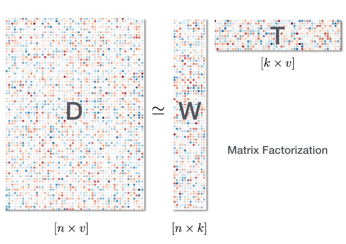
Matrix factorization is an important component of collaborative-filtering based approaches of recommendation systems as it allows us to approximate the original matrix. While this can be compuationally quite demanding it generally pays off, since whenever any matrix multiplication needs to be performed, it can be done much faster due to the reduced size of the matrix after factorization.

It is important to note that matrix factorization is not the end result, but a tool to help reduce the size of the matrix for further computations.

Singular Value Decomposition

In linear algebra, the singular value decomposition (SVD) is a factorization of a real or complex matrix. It is the generalization of the eigendecomposition of a positive semidefinite normal matrix.

Matrix factorization is an important component of collaborative-filtering based approaches of recommendation systems as it allows us to approximate the original matrix.

We say that our original sparse matrix is similar to a linear map, and thus can make algorithms that predict how people rate beers with surprisingly good accuracy. So if you know that a beer such as Blue Moon gets ratings low reviews from a certain group of users, then a new person may review Blue Moon based on a linear combination of how well they align with that group of people, if they strongly align, the model will predict a low rating for Blue Moon. By “align" I mean the user has similar ratings across other beers to the users in the group. In other words, a linear combination of users epitomize the process of rating beers.

SVD provides an useful approach to matrix factorization that represents the process of people rating beers. By changing the basis of one or both vector spaces involved, we isolate the different (orthogonal) characteristics of the process. In the context of our movie example, “factorization” means the following:

Come up with a basis set of vectors v₁, v₂, ..., v_i so that every beer can be written as a linear combination of the v_i.

Do the analogous thing for people to get a basis set for beer drinkers.

Do steps 1 and 2 in such a way that the map \(\Sigma \) is diagonal with respect to both new bases simultaneously.

One might think of the v_i as “idealized beers" and the p_j as “idealized beer drinkers”. For example, an “idealized beer" may be a stout, and its corresponding “idealized beer drinker" may be someone that only drinks stouts, though its unlikely the "idealized beer" will fall into categories corresponding to types of beers.

Alternating Least Squares

The algorithmn of alternating least square aims to factorize the original matrix and obtain two matrices similar to \(W \) and \(T \) that were obtained using SVD. To do this we first estimate \(W \) using a random initialization of \(T \) and estimate \(T \) by using \(W \) . After enough number of iterations, we should hopefully reach convergence where either the matrices \(W \) and \(T \) are no longer changing or the change is below some tolerance.

def alternating_least_squares(Cui, factors, regularization=0.01,
                              iterations=15, use_native=True, num_threads=0,
                              dtype=np.float64):
    """ factorizes the matrix Cui using an implicit alternating least squares
    algorithm
    Args:
        Cui (csr_matrix): Confidence Matrix
        factors (int): Number of factors to extract
        regularization (double): Regularization parameter to use
        iterations (int): Number of alternating least squares iterations to
        run
        num_threads (int): Number of threads to run least squares iterations.
        0 means to use all CPU cores.
    Returns:
        tuple: A tuple of (row, col) factors
    """
    #_check_open_blas()

    users, items = Cui.shape

    X = np.random.rand(users, factors).astype(dtype) * 0.01
    Y = np.random.rand(items, factors).astype(dtype) * 0.01

    Cui, Ciu = Cui.tocsr(), Cui.T.tocsr()

    solver = least_squares

    for iteration in range(iterations):
        s = time.time()
        solver(Cui, X, Y, regularization, num_threads)
        solver(Ciu, Y, X, regularization, num_threads)
        print "finished iteration %i in %s" % (iteration, time.time() - s)

    return X, Y


def least_squares(Cui, X, Y, regularization, num_threads):
    """ For each user in Cui, calculate factors Xu for them
    using least squares on Y.
    Note: this is at least 10 times slower than the cython version included
    here.
    """
    users, factors = X.shape
    YtY = Y.T.dot(Y)

    for u in range(users):
        # accumulate YtCuY + regularization*I in A
        A = YtY + regularization * np.eye(factors)

        # accumulate YtCuPu in b
        b = np.zeros(factors)

        for i, confidence in nonzeros(Cui, u):
            factor = Y[i]
            A += (confidence - 1) * np.outer(factor, factor)
            b += confidence * factor

        # Xu = (YtCuY + regularization * I)^-1 (YtCuPu)
        X[u] = np.linalg.solve(A, b)

factors = 50
als_user_factors, als_beer_factors = alternating_least_squares(bm25_weight(train_data), factors)
als_ii = TopRelated_itemitem(als_beer_factors.T)

Implicit Matrix Factorization

Defined by:

• No negative feedback - entries must be positive.

• Inherently noisy - For example, someone may drink a lot of PBR, because it is cheap, rather than because they like it.

• While numerical value of explicit feedback indicates preference, the numerical value of implicit feedback indicates confidence that a user prefers an item.

Code can be found from Chris Johnson's blog here, based on this paper, and demonstrated below:

class ImplicitMF():

    def __init__(self, counts, num_factors=40, num_iterations=30,
                 reg_param=0.8):
        self.counts = counts
        self.num_users = counts.shape[0]
        self.num_items = counts.shape[1]
        self.num_factors = num_factors
        self.num_iterations = num_iterations
        self.reg_param = reg_param

    def train_model(self):
        self.user_vectors = np.random.normal(size=(self.num_users,
                                                   self.num_factors))
        self.item_vectors = np.random.normal(size=(self.num_items,
                                                   self.num_factors))

        for i in xrange(self.num_iterations):
            t0 = time.time()
            print 'Solving for user vectors...'
            self.user_vectors = self.iteration(True, csr_matrix(self.item_vectors))
            print 'Solving for item vectors...'
            self.item_vectors = self.iteration(False, csr_matrix(self.user_vectors))
            t1 = time.time()
            print 'iteration %i finished in %f seconds' % (i + 1, t1 - t0)

    def iteration(self, user, fixed_vecs):
        num_solve = self.num_users if user else self.num_items
        num_fixed = fixed_vecs.shape[0]
        YTY = fixed_vecs.T.dot(fixed_vecs)
        eye1 = eye(num_fixed)
        lambda_eye = self.reg_param * eye(self.num_factors)
        solve_vecs = np.zeros((num_solve, self.num_factors))

        t = time.time()
        for i in xrange(num_solve):
            if user:
                counts_i = self.counts[i].toarray()
            else:
                counts_i = self.counts[:, i].T.toarray()
            CuI = diags(counts_i, [0])
            pu = counts_i.copy()
            pu[np.where(pu != 0)] = 1.0
            YTCuIY = fixed_vecs.T.dot(CuI).dot(fixed_vecs)
            YTCupu = fixed_vecs.T.dot(CuI + eye1).dot(csr_matrix(pu).T)
            xu = spsolve(YTY + YTCuIY + lambda_eye, YTCupu)
            solve_vecs[i] = xu
            if i % 1000 == 0:
                print 'Solved %i vecs in %d seconds' % (i, time.time() - t)
                t = time.time()

        return solve_vecs

Other Methods

Incorporating other user and item features with collaborative filtering are known as hybrid recommender systems. An example of how to incorporate features into your recommendation has been handled by the folks at Lyst with their python package LightFM.

from lightfm import LightFM
model = LightFM(loss='warp')
model.fit(train_data, epochs=30, num_threads=2, user_features=None, item_features=None)

Validation

M-fold validation

A common strategy for splitting recommendation data into training and test sets is leave-k-out. Here, a split percentage is chosen (e.g., 80% train, 20% test) and the test percentage is selected randomly from the user-item pairs with non-zero entries.

Miss-k-out

Miss-k-out involves removing k items from the training set and attempting to predict them

A useful variant that combines leave-k-out and standard K-fold cross validation is (sometimes) called M-fold cross validation. The idea is simple - split the data into a training set and holdout set. On the holdout set, perform leave-k-out.

Evaluation Metrics

Mean Average Precision

This is simply the mean across all users of the average precision at k. The average precision at k (AP@k) is defined as:

For example if the evaluation metric were MAP@100, the recommendation system chooses 100 beers, and its trying to predict a number of beers, \(n \) that have been left out for validation. If the missing beers are correctly choosen and ranked highly in the list of 100, the MAP will be close to 1. If they were not in the list whatsoever, the MAP would be 0.

def apk(actual, predicted, k=10):
    """
    Computes the average precision at k.
    This function computes the average prescision at k between two lists of
    items.
    Parameters
    ----------
    actual : list
             A list of elements that are to be predicted (order doesn't matter)
    predicted : list
                A list of predicted elements (order does matter)
    k : int, optional
        The maximum number of predicted elements
    Returns
    -------
    score : double
            The average precision at k over the input lists
    """
    if len(predicted)>k:
        predicted = predicted[:k]

    score = 0.0
    num_hits = 0.0

    for i,p in enumerate(predicted):
        if p in actual and p not in predicted[:i]:
            num_hits += 1.0
            score += num_hits / (i+1.0)

    if not actual:
        return 0.0

    return score / min(len(actual), k)

def mapk(actual, predicted, k=10):
    """
    Computes the mean average precision at k.
    This function computes the mean average prescision at k between two lists
    of lists of items.
    Parameters
    ----------
    actual : list
             A list of lists of elements that are to be predicted 
             (order doesn't matter in the lists)
    predicted : list
                A list of lists of predicted elements
                (order matters in the lists)
    k : int, optional
        The maximum number of predicted elements
    Returns
    -------
    score : double
            The mean average precision at k over the input lists
    """
    return np.mean([apk(a,p,k) for a,p in zip(actual, predicted)])
    

Normalized Discounted Cumulative Gain

The normalized discounted cumulative gain (NDCG) is similar to the MAP, however strongly emphasizes that items with high relevance should be placed early in the ranked list, and that order is important.

The NDCG@k is the normalised result of DCG@k so we can obain a value beween 0 and 1.

def dcg_at_k(r, k, method=0):
    """Score is discounted cumulative gain (dcg)
    Relevance is positive real values.  Can use binary
    as the previous methods.
    Code source: https://gist.github.com/bwhite/3726239
    Example from
    http://www.stanford.edu/class/cs276/handouts/EvaluationNew-handout-6-per.pdf
    >>> r = [3, 2, 3, 0, 0, 1, 2, 2, 3, 0]
    >>> dcg_at_k(r, 1)
    3.0
    >>> dcg_at_k(r, 1, method=1)
    3.0
    >>> dcg_at_k(r, 2)
    5.0
    >>> dcg_at_k(r, 2, method=1)
    4.2618595071429155
    >>> dcg_at_k(r, 10)
    9.6051177391888114
    >>> dcg_at_k(r, 11)
    9.6051177391888114
    Args:
        r: Relevance scores (list or numpy) in rank order
            (first element is the first item)
        k: Number of results to consider
        method: If 0 then weights are [1.0, 1.0, 0.6309, 0.5, 0.4307, ...]
                If 1 then weights are [1.0, 0.6309, 0.5, 0.4307, ...]
    Returns:
        Discounted cumulative gain
    """
    r = np.asfarray(r)[:k]
    if r.size:
        if method == 0:
            return r[0] + np.sum(r[1:] / np.log2(np.arange(2, r.size + 1)))
        elif method == 1:
            return np.sum(r / np.log2(np.arange(2, r.size + 2)))
        else:
            raise ValueError('method must be 0 or 1.')
    return 0.


def ndcg_at_k(r, k, method=0):
    """Score is normalized discounted cumulative gain (ndcg)
    Relevance is positive real values.  Can use binary
    as the previous methods.
    Code source: https://gist.github.com/bwhite/3726239
    Example from
    http://www.stanford.edu/class/cs276/handouts/EvaluationNew-handout-6-per.pdf
    >>> r = [3, 2, 3, 0, 0, 1, 2, 2, 3, 0]
    >>> ndcg_at_k(r, 1)
    1.0
    >>> r = [2, 1, 2, 0]
    >>> ndcg_at_k(r, 4)
    0.9203032077642922
    >>> ndcg_at_k(r, 4, method=1)
    0.96519546960144276
    >>> ndcg_at_k([0], 1)
    0.0
    >>> ndcg_at_k([1], 2)
    1.0
    Args:
        r: Relevance scores (list or numpy) in rank order
            (first element is the first item)
        k: Number of results to consider
        method: If 0 then weights are [1.0, 1.0, 0.6309, 0.5, 0.4307, ...]
                If 1 then weights are [1.0, 0.6309, 0.5, 0.4307, ...]
    Returns:
        Normalized discounted cumulative gain
    """
    dcg_max = dcg_at_k(sorted(r, reverse=True), k, method)
    if not dcg_max:
        return 0.
    return dcg_at_k(r, k, method) / dcg_max
  

Best Practices

Recommendation problems can be fun, but tough to evaluate. It's important to absorb the points above, and think about what approaches make the most sense for your situation.

Giving advice that will work generically is hard, but the following list will probably cover best practices is most situations:

• Think carefully about the right strategy for splitting your data. Leave-k-out is simple, but may not be well-suited to data which has many users with few entries. M-fold is a good representation of your final model, but may require enough data and available computation.

• Metrics should be chosen with the end goal in mind. Error and classification metrics are good for assessing overall performance, but if recommending N items, one should at least consider rank-based metrics.

• Know the details of metrics, be able to provide a plain language explaination and justify your choices.

• When practically feasible, check that your metrics are statistically significant when comparing different models. You may need to run more train/test experiments.

• It's always a good idea to examine how metrics vary with subgroups of the data. For example, how does a given metric change for users with few item entries versus those with lots.

• Convince your audience - explain the metrics, but help them connect. Qualitative approaches can help here.

Let's Drink - Choose Your Beer